icclim called from OpenClimateGIS - Examples

icclim indices (ECA&D climate indices) are implemented in the OpenClimateGIS (Version 1.1.0) Python package.

import ocgis

rd = ocgis.RequestDataset("tas_19800101_19891231.nc", variable="tas")

It is also possible to pass a list of datasets:

rd = ocgis.RequestDataset(
    ["tas_19800101_19891231.nc", "tas_19900101_19991231.nc"], variable="tas"
)

Subsetting with time_range and/or time_region

Note

See ocgis time_range doc and ocgis time_region doc.

For temporal subsetting we use the time_range parameter:

import datetime

dt1 = datetime.datetime(1985, 1, 1)
dt2 = datetime.datetime(1995, 12, 31)
rd = ocgis.RequestDataset(
    ["tas_19800101_19891231.nc", "tas_19900101_19991231.nc"],
    variable="tas",
    time_range=[dt1, dt2],
)

or/and the time_region parameter:

rd = ocgis.RequestDataset(
    ["tas_19800101_19891231.nc", "tas_19900101_19991231.nc"],
    variable="tas",
    time_region={"month": [6, 7, 8]},
)

rd = ocgis.RequestDataset(
    ["tas_19800101_19891231.nc", "tas_19900101_19991231.nc"],
    variable="tas",
    time_region={"year": [1989, 1990, 1991], "month": [6, 7, 8]},
)

Temporal aggregation with calc_grouping

Note

See ocgis calc_grouping doc.

Annual values:

calc_grouping = ["year"]

Monthly values:

calc_grouping = ["year", "month"]  # or calc_grouping = ['month', 'year']

Seasonal values:

spring = [[3, 4, 5], "unique"]  # spring season (MAM)
summer = [[6, 7, 8], "unique"]  # summer season (JJA)
autumn = [[9, 10, 11], "unique"]  # autumn season (SON)
winter = [[12, 1, 2], "unique"]  # winter season (DJF)
long_winter = [[10, 11, 12, 1, 2, 3], "unique"]  # winter half-year (ONDJFM)
long_summer = [[4, 5, 6, 7, 8, 9], "unique"]  # summer half-year (AMJJAS)

Example 1: simple indice calculation

The example below will create a netCDF file “indiceTG_1985_1995.nc” containing TG indice:

calc_icclim = [{"func": "icclim_TG", "name": "TG"}]
ops = ocgis.OcgOperations(
    dataset=rd,
    calc=calc_icclim,
    calc_grouping=calc_grouping,
    prefix="indiceTG_1985_1995",
    output_format="nc",
    add_auxiliary_files=False,
)
ops.execute()

Example 2: multivariable indice calculation

To calculate an indice based on 2 variables:

rd_tasmin = ocgis.RequestDataset(tasmin_19800101_19891231.nc, "tasmin")
rd_tasmax = ocgis.RequestDataset(tasmax_19800101_19891231.nc, "tasmax")
rds = [rd_tasmin, rd_tasmax]
calc_grouping = ["year", "month"]
calc_icclim = [
    {
        "func": "icclim_ETR",
        "name": "ETR",
        "kwds": {"tasmin": "tasmin", "tasmax": "tasmax"},
    }
]
ops = ocgis.OcgOperations(
    dataset=rds,
    calc=calc_icclim,
    calc_grouping=calc_grouping,
    prefix="indiceETR_1980_1989",
    output_format="nc",
    add_auxiliary_files=False,
)
ops.execute()

Example 3: percentile-based indices

Calculation of percentile-based indices is more complicated. The example below shows how to calculate the TG10p indice.

dt1 = datetime.datetime(1980, 1, 1)
dt2 = datetime.datetime(1989, 12, 31)
time_range_indice = [dt1, dt2]  # we will calculate the indice for 10 years
rd = ocgis.RequestDataset(tas_files, "tas", time_range=time_range_indice)
basis_indice = rd.get()  # OCGIS data object

We do the same for reference period (usually the reference period is the 1961-1990 (30 years)):

dt1_ref = datetime.datetime(1961, 1, 1)
dt2_ref = datetime.datetime(1990, 12, 31)
time_range_ref = [dt1_ref, dt2_ref]
rd_ref = ocgis.RequestDataset(tas_files, "tas", time_range=time_range_ref)
basis_ref = rd_ref.get()  # OCGIS data object

To get the 10th daily percentile basis of the reference period:

values_ref = basis_ref.variables["tas"].value
temporal = basis_ref.temporal.value_datetime
percentile = 10
width = 5  # 5-day window
from ocgis.calc.library.index.dynamic_kernel_percentile import (
    DynamicDailyKernelPercentileThreshold,
)

daily_percentile = DynamicDailyKernelPercentileThreshold.get_daily_percentile(
    values_ref, temporal, percentile, width
)  # daily_percentile.shape = 366

Finally, to calculate the TG10p indice:

calc_grouping = ["year", "month"]  # or other
kwds = {
    "percentile": percentile,
    "width": width,
    "operation": "lt",
    "daily_percentile": daily_percentile,
}  # operation: lt = "less then", beacause we count the number of days < 10th percentile
calc = [{"func": "dynamic_kernel_percentile_threshold", "name": "TG10p", "kwds": kwds}]
ops = ocgis.OcgOperations(
    dataset=rd,
    calc_grouping=calc_grouping,
    calc=calc,
    output_format="nc",
    prefix="indiceTG10p_1980_1989",
    add_auxiliary_files=False,
)
ops.execute()

Example 4: OPeNDAP dataset, big request

If you want to process OPeNDAP datasets of total size more than for example the OPenDAP/THREDDS limit (500 Mbytes), use the compute function which processes data chunk-by-chunk:

from ocgis.util.large_array import compute

This function takes the tile_dimention parameter, so first we need to find an optimal tile dimention (number of pixels) to get a chunk less than the the OPenDAP/THREDDS limit:

limit_opendap_mb = (
    475.0  # we reduce the limit on about 25 Mbytes (don't ask me why :) )
)
size = ops.get_base_request_size()
nb_time_coordinates_rd = size["variables"]["tas"]["temporal"]["shape"][0]
element_in_kb = size["total"] / reduce(
    lambda x, y: x * y, size["variables"]["tas"]["value"]["shape"]
)
element_in_mb = element_in_kb * 0.001
import numpy as np

tile_dim = np.sqrt(
    limit_opendap_mb / (element_in_mb * nb_time_coordinates_rd)
)  # maximum chunk size

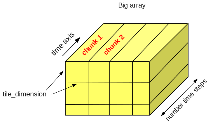
Note

Chunks are cut along the time axis, i.e. a maximum chunk size in pixels is tile_dimention x tile_dimention x number_time_steps.

Now we can use the compute function:

rd = ocgis.RequestDataset(input_files, variable="tas", time_range=[dt1, dt2])
ops = ocgis.OcgOperations(
    dataset=rd,
    calc=calc_icclim,
    calc_grouping=calc_grouping,
    prefix="indiceETR_1980_1989",
    add_auxiliary_files=False,
)
compute(ops, tile_dimension=tile_dim)